Discussion of program transformations and laziness

Extensions and imports for this Literate Haskell file

module ControlFlowDemo where

import LazyPPL
import LazyPPL.SingleSite
import LazyPPL.Distributions
import Control.Monad
import Graphics.Matplotlib

We consider a simple but slightly contrived model to illustrate how control flow transformations and laziness can be advantageous. Our first prior on pairs of booleans.

prior1 :: Prob (Bool,Bool)
prior1 = 
  do x <- bernoulli 0.5
     y <- if x then bernoulli 0.4 else bernoulli 0.7
     return (x,y)

Our model conditions on the two booleans being equal. This means that if x changes, y has to change too, and vice versa.

model :: Prob (Bool,Bool) -> Meas Bool
model prior =
  do (x,y) <- sample prior
     score (if x==y then 1 else 0)
     return x

The posterior probability of (model prior1) returning true is 4/7.

Since x and y are correlated, it is not a good idea to use a naive Metropolis Hastings simulation. But this is an extreme example, and less extreme examples might appear in more complex probabilistic programs that do benefit from Metropolis Hastings simulation, where the correlations are not known in advance.

Here is a second implementation of the prior. It is mathematically equivalent, and computationally equivalent on each run, because of laziness. With Metropolis-Hastings, it is asymptotically the same (of course, as long as the proposal is irreducible – see below). But in practice this prior works better with Metropolis-Hastings because it explicitly uses different sites for the two different conditional branches.

prior2 :: Prob (Bool,Bool)
prior2 =
  do x <- bernoulli 0.5
     ytrue <- bernoulli 0.4
     yfalse <- bernoulli 0.7
     return (if x then (x,ytrue) else (x,yfalse))

Of course, we could solve this particular program analytically. The point is rather that we have a universal program transformation manipulation that could be applied automatically.

The following chart shows that the effective sample size (the ratio between the variance of a single true sample and the variance among the generated samples) is much better with this second implementation of the prior, although Metropolis Hastings is still far from optimal for this contrived problem.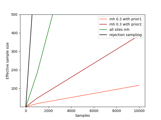

(Code for precision of estimators)

-- Take a sampler (m)  returning reals, regarded as an estimator,
-- and calculate the mean and precision for the estimator.
-- k is the number of samples to use in the estimator.
-- n is the number of runs to average over to approximate the mean, variance and ess.
meanPrec :: IO [(Double,a)] -> Int -> Int -> IO (Double,Double)
meanPrec m n k =
  do xwss <- replicateM n m
     let as = map ((\x -> x / (fromIntegral k)). sum . map fst . take k) xwss
     let mean = (sum as) / (fromIntegral n) -- sample mean
     let var = (sum (map (\x -> (x - mean)^2) as)) / (fromIntegral n) -- sample variance
     return (mean,1/var)

(Plotting code)

plotESSA = 
  do putStrLn "Plotting images/controlflow-essA.png..."
     let xs = [1,1000,10000]
     -- A rejection sampler where the scores are known to be 0 or 1.
     let rejectionsampler m = fmap (filter (\(_,w) -> w>0.00001)) $ weightedsamples $ m
     let truevar = (4.0/7.0) - (4.0/7.0)^2 -- variance for one true sample
     -- Tests to plot
     as <- forM xs $ fmap (\(_,prec)->truevar*prec) . meanPrec (mh 0.3 $ fmap fromBool $ model prior1) 100
     cs <- forM xs $ fmap (\(_,prec)->truevar*prec) . meanPrec (mh 0.33 $ fmap fromBool $ model prior2) 100
     es <- forM xs $ fmap (\(_,prec)->truevar*prec) . meanPrec (mh 1 $ fmap fromBool $ model prior1) 100
     fs <- forM xs $ fmap (\(_,prec)->truevar*prec) . meanPrec (rejectionsampler $ fmap fromBool $ model prior1) 100
     file "images/controlflow-essA.png" $
       plot xs as @@ [o2 "label" "mh 0.3 with prior1", o2 "color" "tomato"] %
       plot xs cs @@ [o2 "label" "mh 0.3 with prior2", o2 "color" "firebrick"] %
       plot xs es @@ [o2 "label" "all sites mh", o2 "color" "forestgreen"] %
       plot xs fs @@ [o2 "label" "rejection sampling", o2 "color" "black"] %
       ylim (1::Double) (500::Double) %
       xlabel "Samples" % ylabel "Effective sample size" % legend @@ [o2 "loc" "upper right"]
     putStrLn "done."

Irreducibility

This example also illustrates the issue with potential irreducibility in single-site Metropolis Hastings (mh1): the first implementation of the prior is especially bad, because all proposals will be rejected except perhaps one. This irreducibility arises from the hard constraints (scores of 0) and is avoided to some extent with a softer constraint:

softModel :: Prob (Bool,Bool) -> Meas Bool
softModel prior =
  do (x,y) <- sample prior
     score (if x==y then 0.9 else 0.1)
     return x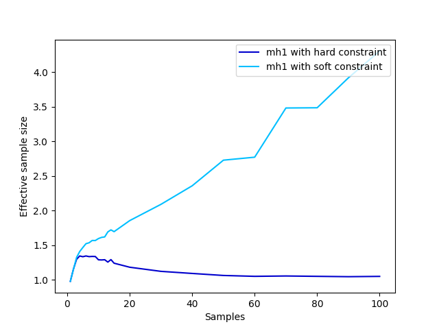

(Plotting code)

fromBool b = if b then 1.0 else 0.0
plotESSB = 
  do putStrLn "Plotting images/controlflow-essB.png..."
     let xs = [1,2,3,4,5,6,7,8,9,10,11,12,13,14,15,20,30,40,50,60,70,80,90,100]
     let truevar = (4.0/7.0) - (4.0/7.0)^2 -- variance for one true sample
     -- Tests to plot
     as <- forM xs $ fmap (\(_,prec)->truevar*prec) . meanPrec (mh1 $ fmap fromBool $ model prior1) 1000 
     bs <- forM xs $ fmap (\(_,prec)->truevar*prec) . meanPrec (mh1 $ fmap fromBool $ softModel prior1) 1000
     file "images/controlflow-essB.png" $
       plot xs as @@ [o2 "label" "mh1 with hard constraint", o2 "color" "mediumblue"] %
       plot xs bs @@ [o2 "label" "mh1 with soft constraint", o2 "color" "deepskyblue"] %
       xlabel "Samples" % ylabel "Effective sample size" % legend @@ [o2 "loc" "upper right"]
     putStrLn "done."

Note about different Metropolis-Hastings kernels in general

These are contrived examples and the reader should not conclude that all-sites Metropolis-Hastings outperforms the more complex Metropolis-Hastings algorithms of LazyPPL in general. To emphasise this, we plot the precision in the intercept for a linear regression example (similar to here).

linreg :: Meas (Double,Double)
linreg =
  do
    a <- sample $ normal 0 3
    b <- sample $ normal 0 3
    let dataset = [(0,5), (0.1,10), (0.2,0)]
    mapM (\(x, y) -> score $ normalPdf (a*x + b) 0.5 y) dataset
    return (a,b)

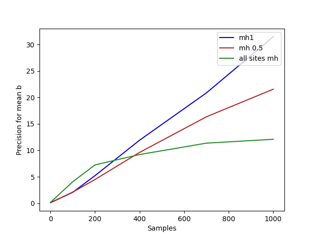
(Here we plot precision, which is proportional to effective sample size, because a general effective sample size analysis isn’t written yet.)

(Plotting code)

plotPrec = 
  do putStrLn "Plotting images/controlflow-prec.png..."
     let xs = [1,100,200,400,700,1000]
     -- Tests to plot
     as <- forM xs $ fmap snd . meanPrec (mh 0.5 $ fmap snd $ linreg) 1000
     bs <- forM xs $ fmap snd . meanPrec (mh1 $ fmap snd $ linreg) 1000
     es <- forM xs $ fmap snd . meanPrec (mh 1 $ fmap snd $ linreg) 1000
     file "images/controlflow-prec.png" $
       plot xs bs @@ [o2 "label" "mh1", o2 "color" "mediumblue"] %
       plot xs as @@ [o2 "label" "mh 0.5", o2 "color" "firebrick"] %
       plot xs es @@ [o2 "label" "all sites mh", o2 "color" "forestgreen"] %
       xlabel "Samples" % ylabel "Precision for mean b" % legend @@ [o2 "loc" "upper right"]
     putStrLn "done."

(Epilogue code)

main = do
  plotESSA
  plotESSB
  plotPrec

Generated by Pandoc from Literate Haskell. Full source on .